Data Vault modelling

Ever heard about Data Vault (DV) Modelling approach?  I'll present here some key elements related to the data modelling aspect of this approach invented by Dan Linstedt. For those interested in learning more, you can also check out Dan's freely available educational video.

The modelling technique proposed can leverage one of the advantage going to higher normalization in data warehousing (DWH) schema, i.e. provide more flexibility against data model changes in source. In the era where adapting to changes is our prime requirement in any IT system (if not the only one!), anyone involved in DWH and BI, will clearly see the advantage of this modelling technique when applied to the DWH data integration layer. Not only can you integrate more data from more OLTP's source systems easily, you also can better adapt to data model changes frequently occurring in these OLTPs.


DV modelling is going toward this trend, but we can also see more extreme case where some people suggest the ultimate flexibility with a 6th Normal Form data model (6NF), see Anchor Modelling as a good example of this.   Obviously, the price to pay for this flexibility is the explosion of number of tables.... which may be a serious challenge for your EDW, depending on your database engine limitations, data volume, complexity of joins needed to support on-going BI activities, etc.

DV Concepts:

In a very distilled definition, the DV is a simple relational data structure highly normalized and meant to store and preserve "100% of data content 100% of the time" from one or more OLTP data source.  The structural modelling has a simple semantic composed of 3 Component (or entity) types: 1- Hub; 2- Link; 3- Satellite.

Key features highlighted by the DV community include:

1. “Detail-oriented, historical tracking and uniquely linked set of normalized tables” : hybrid approach in-between pure 3NF and dimensional model to store and preserve all detail and atomic data changes done in operation database   
2. Flexibility, Scalability and Evolutive to data model changes  made possible by separating data structure from data content (more on that below)
3. Well suited to near real-time and Massively Parallel Processing (MPP) due to, among any reasons, DML involved are pure Insert (some Update can occur depending on your Satellite implementation choice), and Hubs/Links simplified structure (very narrow row)
4. Easy to comprehend and to model:  only limited number of entity type and clear semantic associated to each entity type
5. Precise and definite normalization applicable for modelling any type of data source while making use of relational concepts

Main proponents argue it is suited to be your integrated layer of the EDW (Enterprise Data warehouse) and thus the main data source for all Star Schema/Datamart and other Delivery Layer components sitting closer to Business.   I will not challenge this here as I would need a lot more hands-on experience using DV modelling.  So I’ll simply describe the data modelling aspect, which to me, makes perfect sense for your data historical, auditing and trace-ability needs (if not for other needs)!   


The meta-model model shown next, depicts each Entity type along with their relationship and characteristics:

1- Hub:  one Hub is represented by a single table storing identifiable Entity as found in various functional areas of enterprise data.  In other words, these Hubs represent conceptual understanding of your business entities throughout your business line. Examples of these business entities are

• Customer, Subscriber, Product, Account, Party, Order, Call, Invoice, Part, Employee, Purchase order, Service, Inventory, Material, ... (this list getting huge with Corporation acquisition and portfolio growth...)

And example of business lines are 

• Sales, Marketing, HR, Finance, Planning, Strategy, Production, Manufacturing, Contracting, etc.

As such these concepts are commonly found and stored in one form or another within all the OLTP systems (i.e. disparate, non-integrated, non-conformed, duplicated..) and we intend to centrally them in our DV repository by first integrate their Keys into Hub.

It must have one or more natural/business keys that allow for unique identification, so Hubs represent the Primary-Keys of our business data, in effect separating structure (Hubs) from the content (Satellite) resulting in better flexibility!  Nothing else is stored there, no parent-child relation, no textual info, they must have no other dependencies than themselves. These can then be loaded (near real-time) as "observed" in all OLTP systems without worrying about lookups and relationship constraint.

Typically in Dimensional world, this would be similar to Dimension-keys, but not necessarily as we could also have a Fact table with fact (or transaction) identifiable through natural keys (we would then accompany this particular fact-Hub with a Link structure to capture all many-to-many relationships found in star schema).   

Hub Attributes:

1. Business key(s) (mandatory) natural composite or single key as used by business people/operational system during operations
2. Surrogate Key (*optional according to DV documentation, but surely mandatory especially when used in the context of DWH integrated data). Here the definition of Surrogate key is a bit misleading in all info found, but personally I see three different levels:
• 1. 1. OLTP Surrogate-key provided by source system (most entities cannot be tracked down correctly in time using only business keys, OLTP data models already acknowledged that by using own surrogate-key)
• 1. 2. DV Surrogate-key created by the DV repository: the unique Sequence Id usable as valid PK in the Hub table ( independent and unique across all system source)
• 1. 3. EDW-key (not unique), that would be used to merge and identify same entities across system sources (first level of integration, as suggested in my comments section at end of doc)
3. Loading timestamp (mandatory) audit data recording when data was inserted
4. Record source (mandatory) the system operational source used for traceability and integration purposes.

2- Link: one Link is represented by a single table storing relationship data between two or more Hub entities (Link could used to connect other Links as well).  They represent associations, relationship or links among your Business Entities (contained in Hub). These can change over time, and my or my not have direction (directed from-to).

Instantiated as a separate table, Link can thus support any many-to-many 3NF relationships (i.e. in source system, the relationships between business entity can be of any cardinality types: 1-to-1, n-to-1 or n-to-m) and flexible to support future changes of Cartesian rules.  Hence, in source system any FK relationship is a good candidate for Link.  The constraint on cardinality types will not be enforced by the database (as all relationship are now modelled as many-.to-many physical structure) but rather the ETL tools, which is typically found on DWH implementation.

Note that Hubs should all have association captured by Links (isn’t it the role of any process to perform some kind of association among business entities), otherwise they would be considered Stand-alone tables and not Hubs (see point 5 below).

Typically in Dimensional world, this would be similar to Fact table.  We normally source Link entity from transactional-data in source system, as each transaction is characterized by a few entities, but again, the transaction itself could be represented separately in a Hub.   The relevant point is whether the entity is identifiable through business keys, for example transactions could be identified through a unique recognized transaction-Ids ticket.

Link Attributes:

1. Hub Surrogate FK Keys (mandatory) Business sequence keys giving the linkage back to each Hub unique Entity (at minimum 2 Entities). These do not correspond to the Hub business natural keys but rather the Surrogate key (can be the OLTP or the DM level key ...depending on the context, but safer to go with the real DM-level surrogate key)
2. Link Surrogate Key (*optional according to here) a primary unique key to be considered mandatory in the context of Link connected to other Links, but more importantly, to allow for Context (Satellite) data to relate to Links in a flexible and dynamic way (without being dependent on Links granularity and key changes at source).
3. Loading timestamp (mandatory) audit data recording when relationship was first inserted (observed)
4. Record source (mandatory) the system operational source used for traceability and integration purposes.

Hubs and Links are free of contextual info, they simply provide structural data.  To provide context data, we go to Satellite:  the content data.


3- Satellite: one Satellite is represented by a single table storing the contextual, descriptive and information associated to one Hub or Link entity.    These are the Content-data of our data model as opposed to Structure-data given by Hub and Link.  They must contain some kind of timestamp (an attribute or a numerical sequence pointing to a table that stores these timestamp) used to time frame the observed descriptive data (data valid starting at this given point in time).  

They must also contain a unique n-to-1 FK relationship pointing back to the Hub or Link it describes.    These will obviously contain a large number of textual fields which are all subject to change over time.  As such, Satellites can be defined at grain-level formed by grouping different attributes with similar Rate-of-Change, this will help reducing data redundancy when inserting new rows with updated attributes.      

Typically in Dimensional world, this would be similar to type-2 slowly changing Dimension, where we keep track of all state  of Fact table.

Satellite Attributes:

1. Hub or Link Primary keys (mandatory) FK pointing back to business entity
2. Loading timestamp (mandatory) audit data recording when new Textual data was observed and inserted into the table
3. Surrogate Key (*optional) a unique key probably useful in the context of m-to-m relationships
4. Record source (mandatory) the system operational source used for traceability and integration purposes.

(Optional) 4- Point-in-time: component represented by a single table defined solely to simplify the Querying logic when extracting data from multiple Satellite components (relevant when one Hub entity have many Satellites associated).   It is one of possible solution meant to mitigate the issues involved when querying Satellites components :

1) Limited Time Context by row:  Inside Satellite table, each record is valid during a limited time span given by the current row and the next row.   So to get data content “As-Of” a certain Date, we need to do row-comparison which is cumbersome in SQL (involves sub-select statement to get next row Date).  

2) Satellite entity granularity:  Textual info data will be buried inside multiple Satellite tables, in effect increasing the number of tables to join and with each involving dedicated sub-select statement to get content As-Of given date.

Point-in-time tables ease the SQL processing burden by combining Load Timestamp related to each Satellite of a business entity into a single structure: PIT-table.  Whenever there is a new row inserted from one Satellite, this triggers a new row to be created in the PIT-table, with the Load Timestamp corresponding to the Load Timestamp of the triggering of this particular Sattellite (while keeping timestamp for the other Satellite unchanged).  This PIT-table structure is depicted here: 

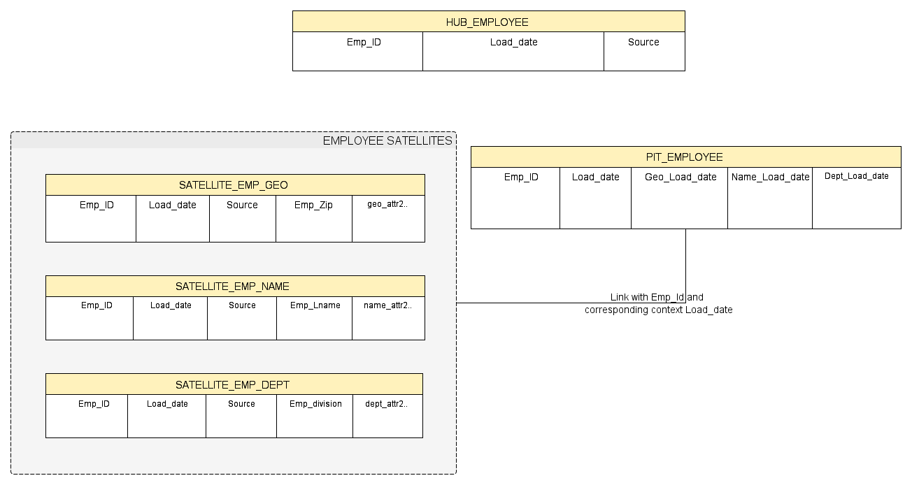
Hence, one wishing to get some Employee name, geo and department info as of “EndOf-lastMonth”, we use the PIT-table to get the right timestamp contextualized by satellite and equi-join with all Satellites needed.  This limit to one the number of sub-select statement as illustrated by the pseudo-SQL code below:

Select pit.emp_id          ,geo.geo_attr2          ,name.name_attr2          ,dept.dept_attr2 From PIT_EMPLOYEE pit Inner join SATELLITE_EMP_GEO geo ON (pit.emp_id = geo.emp_id                                                                    AND pit.geo_load_date = geo.load_date) Inner join SATELLITE_EMP_NAME name ON (pit.emp_id = name.emp_id                                                                    AND pit.name_load_date = name.load_date) Inner join SATELLITE_EMP_DEPT dept ON (pit.emp_id = dept.emp_id                                                                    AND pit.dept_load_date = dept.load_date) Where pit.load_date = (Select max(load_date)                         From PIT_EMPLOYEE p                         Where                         pit.emp_id = p.emp_id                         And p.load_date <= to_date(‘End-Of-lastMonth’))

* could also be implemented with more analytical SQL function (windowing LAG/LEAD), but this would still requires a sub-select statement to get the needed row.



Other alternatives could be proposed that avoid the needs to create these artificial PIT table.  

We could proceed with a slight denormalization on the Satellites table and add an extra timestamp attribute (Loading_date/Loading_close_date) which is fully redundant with next row timestamp.  Then each row would have two timestamp :

1. Loading start timestamp  (i.e. the mandatory Loading timestamp)  
2. Loading close timestamp equals to a far-fetched future date when the present record is still valid (current one), or would equal to the next Loading date when that next record came to replace this present one.

In effect, this replaces the SQL sub-select statement with additional filter conditions (based on timestamp range), as highlighted by the new pseudo-SQL code below:

Select geo.geo_attr2          ,name.name_attr2          ,dept.dept_attr2 From SATELLITE_EMP_GEO geo Inner join SATELLITE_EMP_NAME name ON (name.emp_id = geo.emp_id) Inner join SATELLITE_EMP_DEPT dept ON (dept.emp_id = geo.emp_id) Where to_date(‘End-Of-lastMonth’)) Between geo.load_date And geo.load_close_date  AND to_date(‘End-Of-lastMonth’)) Between name.load_date And name.load_close_date  AND to_date(‘End-Of-lastMonth’)) Between dept.load_date And dept.load_close_date

So the SQL engine no longer needs to process the sub-query (select max(...) ..) but this come at the price of higher complexity during loading with the required update row to end-date satellite row.

Also possible, is what is referred to by D. Linstedt (original creator of DV modelling) as hybrid or combined approach where PIT table is only used as a way to keep current Load timestamp recorded in all Satellites associated to a specific Hub entity.  This new PIT is then refreshed after every load to reflect updated current rows and will contain one load_timestamp field per each satellite table.  So new PIT table becomes handy when it’s time to join with previous current row in order to close (end-dating) their status.   This approach simplifies Querying only when reporting As-of today data, since PIT only keeps current timestamp   There are more issues and difficulties with reporting these data, but this will beyond this introduction doc, please refer to online material.



(Optional) 5- Standalone: component represented by a single table and created to store unrelated Data.   By unrelated, we mean data with no real business identity and no business-related linked with existing Hub, such as look-up and other referential data.  Examples for Stand-alone tables include calendars, time, code and any other descriptive tables.




My Comments on DV:

Let me first say I believe the data modelling aspect is sound and the approach makes sense for what it is : storing non-integrated relational data in a flexible, dynamic, granular and scalable way from any number of OLTP sources.  

However, my concerns are more related to the role that DV data repository presumably could  take... i.e. become your established EDW platform (at least one brick of it).  This role is  promoted  by the community and this is where I definitely  need more hands-done experience with real implementation done on large Enterprise dataset ecosystem.    


If by EDW, we simply mean the staging layer whose role is to consolidate the facts (what and  when), and everything else is contained in downstream Datamart layer (i.e. the interpretation of the data) with the application of business rules (i.e. business view), then it is arguably a right fit for this purpose!!   But then this discussion comes down to what should constitute your EDW.  My view is that it should be more than merely a staging place, so I guess my points below are raised having this concern in mind, but again I hardly saw any real implementation of the DV inside a big EDW environment (may involve a lot more than what is now published by the DV community and made freely available on the net). 


◾ Table Explosion: Data structure modelling rules has important impact on the number of tables created, which is significantly more than the corresponding source OLTP databases and obviously more than a corresponding Dimensional model.      The explosion in number of tables is due to :

1- cost to pay for splitting Structure from Content (Hubs/Link and Satellites)

2- further splitting content by rate-of-change (many satellites for same entity)

3- modelling any relationship as external m-to-m relationships table

As such, the DV modelling is not rightfully suited to direct reporting/online analysis/ad-hoc querying solution implementation.  However, there are techniques modelling that can help circumvent but again at the price of adding more tables.  I guess the real solution is to go optimize your Join processing either through sophisticated DB engine or other means.


◾ ODS alternative: If the DV is simply meant to replace your ODS layer, then I’m not sure it makes sense to re-engineer completely this layer to replace with a full DV.   First hand, it is not overly complex to build new ODS layer as copy of your OLTP data (plus some timestamp and auditing info) by leveraging ETL tools designed to do full Historical Tracking.   So unless, you have stringent requirement for auditing/traceability needs, and that some of your OLTP data models are not suited for building an ODS layer.  


◾  OLTP vs EDW Surrogate Key: Obviously adding the OLTP surrogate key in addition to the business/natural keys makes perfect sense, as typically your natural/business keys are not enough to guarantee the correct and unique mapping with same business entity through time, ex.  -msisdn changes from time to time (in mobile comm. industry); -ban (billing account #) also may change when client changes account type, employee# can change when same employee move or change status....    So if DV is used as a single source of your EDW downstream layer, yes we need these set of surrogate Keys.  

Furthermore, if the goal is to build an Integrated layer of the EDW, then I’d say you also need a deeper level of Surrogate-Key: the EDW-level key!   This new key will serve to identify same entity across all OLTP and other source of data in your enterprise.    For example, the business entity Employee will have many independent operational systems collecting data all using different set of surrogate/natural keys (ranging from nt-login, employee-No, email-adress, so on...).      Adding an EDW-level key will provide you with the first integration hook that ties different entities together (all coming from various OLTP sources).

In this respect, when we load the HUB_EMPLOYEE table,  we could simply add this extra-key  EDW_EMP_KEY to be used by downstream layer where we combine satellites data (across different OLTP source) for the same business entity element (see next point).   And if we work under low latency like in near real-time mode, then to avoid adding concurrent access lock, we could leave these new key as Null, and proceed with special Update in batch-mode during offline window hours.



◾  Can DV be your EDW?  When we model the DV as documented, not much integration is provided as we merely provide a central storage where disparate and unrelated-data is accumulated coming from various OLTP sources.  At best we would simply be piling up Hub entities from different source (source tag) into the same Hub table, but most likely we would be creating own set of unrelated Hubs, Satellite and Link tables per OLTP source.   Although It may be sufficient for your needs, it is not however satisfactory for it to be called your EDW !  



◾  Satellites Granularity: the goal of Satellites is to capture (in batch or near real-time) all data changes at source!   This can be mandatory for auditing/legal reason, but certainly not for Reporting or data analytical purposes (who cares whether the user proceeding with manual data entry keeps  ).  So these fine-grained data will impact the EDW by adding extra-rows in the EDW at timeframe scale usually not relevant for most Reporting and BI application needs.



◾ Hub Record deletion : What happen with records are being removed in general?  Best practices dictate that business entities normally do not simply disappear from operational database (usually expired or invalidated).  But from my experience, in real-life scenario this happens from time to time : who never witnesses a patch executed directly on the operational database with all sort of side effects!.   How should we support this deletion:

1. Add an optional Deletion_Timestamp in the Hub entity

• Adv. : easily spotted when querying data in Hub without checking Satellite and the appropriate timespan
• DisAdv. : would require row update on the Hub (loading no longer pure insertion logic)

2. Add Deletion_flag in Satellite accompanied with the normal Timestamp

• Adv. : leave the loading logic of Hub intact (pure insert)
• DisAdv: Require more complex Satellite query

Either case, this timestamp would only be populated once the record has been “observed” to not exist anymore in the source, having the advantage to preserve traceability.    I tend to favor solution I, as explained in the Link Record Deletion below.



◾ Link Record deletion : Also what happen with relationship disappearing (and not simply expired or date-ended from the source)?   In other word, what to do with any FK set to Null for a 1-to-m relationship, or a simple deletion of rows in a m-to-m relationship table.   As with the Hub record deletion, we could also propose the Link or Satellite approaches as suggested above.   

In general, I would not favor the Satellite approach, since Satellites are only meant to carry informational fields existing at the source (content).  The Deletion_flag has different semantic and is not sourced directly from existing fields.  Record Deletion correspond more to Structural-type than content-type, and as such this info should be carried inside Hub or Link and not Satellites.  Furthermore, the semantic to expire/ending an entity or a relationship, is often already built-in explicitly in the OLTP database (i.e. expiration_date, or other flags), which will then be carried over the proper Satellites.  So confusion could arise by having these two type of fields in same Satellite.  


◾  Direct reporting or ad-hoc analysis: I don’t think DV modelling should be used for direct reporting solution, at least not without the use of some View or technical-layer providing special Query services.   This is due to the added complexity (large number of tables, added noise stored in Satellites, more complex join or artificial structure needed to circumvent these, etc..) but as well as due to issues that arise when we simply combine (as opposed to integrate) multiple OLTP data sources.   However, DV has a place for the EDW layer focusing on simply storing accurately all data produced by OLTP system without trying to correctly make sense of this data, so in this sense it sort of provides your Staging layer but with full history and completeness.  So surely a good solution for data traceability and legal auditing standpoint and possibly some good ideas toward the EDW.

So if chosen as to provide the data collection and historical layer, then I’d say it makes more sense for organizations that have very small investment on their EDW platform, or else organizations that are ready to decommission their current EDW (and here there are probably tons of reasons justifying doing so!).  I don’t see cost justification on doing a full revamp/resourcing of current ODS or Integrated layer into Data Vault model.



Martin

A Source-to-Target self-documentation system

 
In the BI world, the corporate Data warehouse platform gets often overly complex quite rapidly.   The number of source components increases rapidly to reach nearly thousand of entities: 

-: consider 10-15 different OLTP’s sources each having roughly 10-20 entities worth of interest (tables and views)
-: consider also the few File-based sources each accompanied with one or more feed entities
-: now consider that each one of these source entities will normally result in many components created and stored downstream in various form and for various reason

After these considerations in mind, one can see the explosion of entities any average BI team manage and continue maintaining to keep evolving.  This can result in maintenance nightmare when the team is asked to do deep impact analysis of changes and updates done on existing entities.   As such it is important to keep and maintain some Source-to-Target metadata and documentation.
 
To understand the dependencies from downstream elements to upstream ones, we can store all source-to-target relationships using a form of Directed Graph.   Each node in the graph represents an entity either found in the DWH or outside in the source layers.  These entities can be in different format or type, for ex. in the DBMS they would be table or view, in the source layer they can be of type file, etc…   The directed edge of the Graph represents the dependency relationship between the source and the target entities.   
 
Various relational modelling techniques can be used to store such Directed Graph.  One of the most flexible way is to use one table to store the From-To relation (edge) and another table to store each entity node.  This was done here with the table STK_ENTITY_LINK having two FK relationship pointing to STK_ENTITY_NODE.
 
The rest of this presents such a model that can automatically be maintained and populated by a feeder (actually this was done using a custom-built Java feeder capable of finding dependencies from database metadata, from reading Pl/SQL code, from reading ETL tool metadata, etc.)
 
 
 
DATA MODEL :

 
DATA AUTOMATIC FEED :
The Data feeder is the process responsible in populating/refresh data model.  It provides this service through a metadata table FEEDER_META. A number of use-case are supported for various ways to trigger a feed job. One entry in FEEDER_META will generate one self-contained graph of Entity nodes. However multiple entries may generate multiple over-lapping graphs. It is up to the Data feeder to avoid duplicating entity Node by recognizing identical node through its URI.
Furthermore, the meta-info is generic enough to support potential other use-cases with certain constraints.
 
Key Issues to watch for is How to we define Domain:
- Can link one domain per entry in FEEDER_META, so all graph nodes will be associated to same domain.

• Drawback= nodes in overlapping graph will inherit multiple domains ?

- Can link one domain only for the starting node

• Drawback= another process will need to complement domain for other nodes and make some decision with Domain clashing.

STK_FEEDER_META

Column	Definition	Optional
meta_key	Primary key	N
Meta_name		N
Domain_name	Domain name of the entity nodes. To link the entire graph generated (or alternatively only the starting node) to the domain --see issues to resolve
starting_node_name	Name of the starting enity node	N
starting_node_type	View, KView, Table, File,	N
starting_node_uri	The unique id of the starting node	N
starting_node_key	Surrogate key linking to the starting node once feed process is complete	Y
Feed_usecase	Usecase name supported
Feed_source	Can be package/table, view name, table.., depending on the Feed_usecase
Feed_extract_sql	For use-case Ad-Hoc, used to fecth code to be parsed
Feed_conn_key	Points to connection to be used for
Links_direction
Last_run_date		N
		Y

User-Case 1-View: Graph Feed starting from DB View entity

• § Starting entity-node point : VIEW identification (db,schema,view)
• § Ending entity-node point : First physical tables encounter
• § Rules: Find Ancestors based on USER_DEPENDENCIES metadata table (recursively)
• § Notes:
• § Metadata fields used: connection info, View name

 
User-Case 2-Cube: Graph Feed starting from OLAP Cube

• § Starting entity-node point : Cube identification (db,schema,view + cube_id)
• § Ending entity-node point : First physical tables encounter
• § Rules: Find Ancestors based on USER_DEPENDENCIES metadata table (recursively)
• § Notes: We could also use other OLAP specialized metadata table
• § Metadata fields used: connection info, cube id and name

 
User-Case 3-TablePackage: Graph Feed starting from Physical Table loaded by one PL/SQL package

• § Starting entity-node point : Table identified (db,schema,table)
• § Ending entity-node point : First physical tables encounter
• § Rules: Find Ancestors based on USER_DEPENDENCIES metadata table. To exclude as dependencies the Physical Table identified, but to include all other objects dependencies (recursively), i.e. the process must not stop at View objects but find all base tables.
• § Notes: We must assume that all other REFERENCED objects are ancestors of the identified Table
• § Metadata fields used: connection info, Table name, Package name, domain

 
User-Case 4-TableAd-Hoc: Graph Feed starting from Physical Table loaded by some ad-hoc code (SQL or PL/SQL)

• § Starting entity-node point : Table identified (db,schema,table)
• § Ending entity-node point : All Parsing DB objects encountered
• § Rules: Find Ancestors based on Parsing ad-hoc code fetched by process, and to other objects dependencies (recursively), i.e. the process must not stop at View objects but find all base tables.
• § Notes:
• § Metadata fields used: connection info, K-View name, connection string, code source location

Martin

p.s. For completeness, I include below all DDL needed for the physical data model
 
 
-------------------------- DDL for Data Model ----------------------
create table STK_ENTITY_DOMAIN(
domain_key NUMBER(9),
domain_name VARCHAR2(50), --
domain_desc VARCHAR2(100),
parent_domain_key NUMBER(9),
created_date DATE,
update_date DATE,
constraint pk_domain primary key (domain_key)
);
comment on table STK_ENTITY_DOMAIN is 'Business Domain for classfying entities into logical grouping';
comment on column STK_ENTITY_DOMAIN.domain_name is 'SIP, OC Efficiency, PMO, Prod Operational Source, etc.';
alter table STK_ENTITY_DOMAIN
add constraint fk_parent_domain foreign key (parent_domain_key) references STK_ENTITY_DOMAIN(domain_key);
create table STK_ENTITY_TYPE(
type_key NUMBER(9),
type_name VARCHAR2(50),
type_desc VARCHAR2(100),
type_cat VARCHAR2(50),
constraint pk_entity_type primary key (type_key)
);
comment on column STK_ENTITY_TYPE.type_name is 'View, Table, K-view, File, External table, Portal/Page, Chart (component), KPI, MOLAP cube...';
create table STK_ENTITY_NODE(
node_key NUMBER(9),
entity_name VARCHAR2(50),
entity_uri VARCHAR2(150),
entity_host VARCHAR2(50),
entity_schema VARCHAR2(50),
metadata_key NUMBER(9),
source_id NUMBER(9),
domain_key NUMBER(9) NOT NULL,
entity_type_key NUMBER(9) NOT NULL,
created_date DATE,
update_date DATE,
constraint pk_entity_node primary key (node_key)
);
comment on column STK_ENTITY_NODE.entity_host is 'host name (for file), database instance (for db objects)';
comment on column STK_ENTITY_NODE.entity_schema is 'schema name for db objects';
comment on column STK_ENTITY_NODE.source_id is 'Id used in source for entity (e.g. dashboard_id for KView, dimension_id,..)';
alter table STK_ENTITY_NODE
add constraint fk_node_domain foreign key (domain_key) references STK_ENTITY_DOMAIN(domain_key);
alter table STK_ENTITY_NODE
add constraint fk_entity_type foreign key (entity_type_key) references STK_ENTITY_TYPE(type_key);
create table STK_ENTITY_LINK(
from_node_key NUMBER(9) NOT NULL,
to_node_key NUMBER(9) NOT NULL,
cross_domain CHAR(1), --
created_date DATE,
update_date DATE,
constraint pk_link primary key (from_node_key,to_node_key)
);
comment on column STK_ENTITY_LINK.cross_domain is 'To flag link crossing two diff domain';
alter table STK_ENTITY_LINK
add constraint fk_from_link_node foreign key (from_node_key) references STK_ENTITY_NODE(node_key);
alter table STK_ENTITY_LINK
add constraint fk_to_link_node foreign key (to_node_key) references STK_ENTITY_NODE(node_key);
create table STK_CONNECTION (
connection_key NUMBER(9),
connection_type VARCHAR2(50),
driver_class VARCHAR2(150),
conn_string VARCHAR2(150),
login VARCHAR2(50),
password VARCHAR2(50),
constraint pk_connection primary key (connection_key)
);
comment on column STK_CONNECTION.conn_string is 'Depends on the type of connection, for DB this corresponds to jdbc_url';
-- job trigger shoud point to the db objects that can be used as a source
--should give the detail on how to construct the graph. (code in sql, pl/sql, )
--
create table STK_FEEDER_META(
meta_key NUMBER(9),
meta_name VARCHAR2(50),
domain_name VARCHAR2(50),
starting_node_name VARCHAR2(50),
starting_node_type VARCHAR2(50),
starting_node_uri VARCHAR2(150),
starting_node_key NUMBER(9),
feed_usecase VARCHAR2(50),
feed_source VARCHAR2(50),
feed_extract_sql VARCHAR2(2000),
feed_conn_key NUMBER(9),
links_direction VARCHAR2(10),
last_run_date DATE,
constraint pk_feeder_meta primary key (meta_key)
);
comment on column STK_FEEDER_META.feed_usecase is 'Values: ''1-View'';''2-KView'';''3-TablePackage;''4-TableAd-Hoc'';';
comment on column STK_FEEDER_META.feed_source is 'Can be package/table, view name, table..';
comment on column STK_FEEDER_META.feed_extract_sql is 'For use-case Ad-Hoc, used to fecth code to be parsed';
/* Additional constraint */
--1- to avoid node with self-link
alter table STK_ENTITY_LINK add constraint no_self_link check (from_node_key <> to_node_key);
--2- Should we have a constraint to avoid two-links between the same entities ?
--------------------------------------------------------------------------
insert into STK_ENTITY_TYPE(type_key,type_name,type_cat) values (1,'Table','Database');
insert into STK_ENTITY_TYPE(type_key,type_name,type_cat) values (2,'View','Database');
insert into STK_ENTITY_TYPE(type_key,type_name,type_cat) values (3,'KView','Database');
insert into STK_ENTITY_TYPE(type_key,type_name,type_cat) values (4,'Synonym','Database');
insert into STK_ENTITY_TYPE(type_key,type_name,type_cat) values (5,'Folder','OS');
insert into STK_ENTITY_TYPE(type_key,type_name,type_cat) values (6,'File','OS');
insert into STK_ENTITY_TYPE(type_key,type_name,type_cat) values (7,'Page','Dashboard');
commit;

Cultural gap: Machine Learning vs Traditional stats

About a decade ago there has been a somewhat controversial paper published by L. Breiman which criticizes the current research trend done by classical/traditional stats community.  In a provoking tone, he compared the research done by the traditional stats community (what he called “Data Modeling Culture”) with the one done by newer machine learning community (referred to as “Algorithmic Modeling community”).   Pretty much everyone recognizes the contribution of the later now, especially in the realm of analytical predictive task with very successful algorithm based on some form of Support Vector Machines SVM or the Random Forest (incidentally created by Breiman himself).   Unfortunately Breiman died not so long after his paper so we will never have the chance to hear his reflection about how things turn out to be nowadays. 

I cannot pretend to follow closely the progression of each culture* and know whether the gap is decreasing or reshaping, or yet whether the “Data Modeling Culture” is catching up and keep on updating their mathematical grounding to better leverage the ever increasing computing power/storage resource made available today.  

*as a side note: although I don’t dedicate enough time to it, I always enjoy going back to the rigor and mathematical grounding of the research/academic world especially after having dealt with too much imprecision, fuzziness, and lack of clarity often characterizing the so-called “real” world project ;-)  

However, I guess that Breiman’s paper helped each community in their own way and contributed in widening each other’s point of view.   This point of view is supported by the growing number of researchers & books treating new algorithmic-based techniques from a more theoretical standpoint and using a more inferential perspective (ex includes work from researcher involved in “statistical learning” like Trevor Hastie, Robert Tibshirani, Jerome Friedman,  Vladimir Cherkassky, Filip Mulier.    

So because of this importance, I decided to highlight some of the elements brought up at the time in Breiman’s article.

Difference in Theoretical Approach

In  essence, most problem typically involve one response variable y which is generated through some form of data generation process attributed to nature functions.   In order to either 1) predict future or unseen y or to 2) understand better how nature operates in generating y, we use a set of input variables contained in the vector x, that we believe have some role in the generation of y.   Obviously, there are other more complex considerations here such as 1) data generation mechanism may originate from more than one underlying process,   2) independency assumption of predictors x, 3) co-dependency or inter-dependencies between the x’s, 4) unobserved input variables z affecting the process, 5) causality vs inference, ..etc.   But these aspects were not the focus of the original paper.

The “Data modelling” culture strive with the utilization of a so-called stochastic data model represented as a simplified model used to replace the nature functions involved in generating y.   These simplified data model are characterized by a chosen function along with their set of associated unknown parameters (BTW these parameters can never be observed) and some form of random noise (e) added especially to explain the difference between the predicted value f(x|m,e) and the real outcome y.    Function used can be simple as linear regression, logistic regression, Cox mode, or more complex like Bayesian methods combined with Markov Chain Monte Carlo.  

The “Algorithmic modelling” considers the nature functions far too complex to be usefully and accurately transposed into a simplified model.  As such, their approach is to consider nature as a black-box and their goal is to find an algorithm function af(x) that operate on x to predict y.  The set of algorithm is growing at fast pace and include things like decision trees, neural nets, svm, random forest, etc.

The main argument against each other camp could be summarized using these terms:

• “ Data modeling” camp:   there is no way one can interpret a blackbox with the level of complexity seen in “Algorithm modelling”, whereas ease of interpretability in data model allows for useful information to be revealed.
• “ Algorithmic modeling” camp:   the goal is not interpretability but accurate information, and what’s the level of confidence in the info revealed when data model performed less accurately than “Algorithm modelling” when cross-validated.

Flaws in Data Modelling Culture

A great deal of effort and focus spent in statistical research revolves around Modelling concerns: 

- What model to apply to data?  -What assumption can be made on the model that supposedly generated data? –what Model parameter inference can be done?  What hypothesis testing to apply?   What confidence interval follows on the parameters inferred?  What distribution of residual sum-of-squares and asymptomatic can be derived?  What is the significant level of coefficients on the basis of model? etc..

This focus on data Modelling, as attractive as it is in terms of the mathematics involved, has the downside of switching the analysis emphasis from the Nature’s mechanism in favour to the Model’s mechanism!  This becomes apparent when one, unintentionally, may later confuse or replace the theoretical model with the real nature’s mechanism that lead to generating the data.  Then, bad or even dangerous conclusion could be drawn especially when the chosen “model is a poor emulation of nature”.  

But the attractiveness and intuitiveness of Model are too strong :  what better can you ask than having a “simple and understandable picture of the relationships between input variables and responses” right in front of you? .   These have resulted in many habits or errors made by some fitting data modeller enthusiasm, which lead them to think their models as infallible and represent the truth!  Here are some examples of mistakes or errors involved (with different level of severity):

• At worst, confidence in the Model reaches the point where even basic test such as Residual analysis and Goodness-of-fit test can are even ignored!
• The validity of the form of the model is assumed right or not questionable (for ex. simple linear regression applied without much consideration as whether linearity exist within variables in the underlying data process generator)
• Test of Goodness-of-fit using multiple correlation coefficient only measure how well the model fits the sample of data and nothing to do with the problem at hand.
• Goodness-of-fit test suffer from a number of issues, most of the time, simply ignored :
  1. they have the tendency to not reject linearity unless nonlinearity becomes extreme
  2. they test in every directions leading test to be rarely rejected unless lack of fit is extreme
  3. they are often simply not applicable when model tinkering is done like removal of attribute, or adding nonlinearity by combining attributes/variables
• Residual analysis also has its own limitations:
  1. they cannot uncover lack of fit with more than four to five dimensions!
  2. the interactions between variables produce good residual plots for a number of failed model

Comes next the issue of choice:  what are we supposed to expect by interpreting of a unique model out of potentially many hundreds or thousands!  A direct effect of using a simple yes-no answer to check model goodness is that, implicitly, a number of different Models will be equally as good!  “Data will point with almost equal emphasis on several possible models”.
This is even more relevant nowadays with the sheer number of variables we capture and track and made available to analysis (in the era of Big-data, dataset are much more complex and highly dimensional).   Think of sub-selecting a small number of variables from many available and see how many competing models could we have :   from a pool of 50 variables, how many different subset variables models would compete against each other.  Assuming we’re just looking at the best 5 variables, it becomes a 2.1million problem -->C(50,5) !

The real alternative to Goodness-of-fit is to consider the model predictive accuracy.  This can only be done by applying the function to data from test sample (unused and/or unseen) and compare the model predicted value with the actual measured value, i.e. apply cross-validation!   The closer the two will be the better the model emulates the real process.    This un-biased cross-validation approach (i.e. independent test sample) is the only way to avoid the model to be made to overfit the data at hand and producing overly good predictive accuracy.

Algorithmic Modeling Lessons

In this approach, the focus is shifted from aspects of data modelling to aspects of algorithm’s properties.   These properties range from their “strength” as predictor, their convergent ability (for iterative-type of algo), and their features or capability that made them a good predictor.   
It is interesting to note that in machine learning theory, we usually only have one assumption being imposed on the data process, i.e. that the data is drawn i.i.d. from an unknown multivariate distribution!

The author goes on to describe in more details two of these particularly good predictor (SVM and Random forest) and compare them with other traditional procedure in the context of real and well known research data set.   Not surprisingly, the results all favour the  “Algorithmic modelling” techniques with sometimes large improvement in predictive accuracy.  

I’m not going to present the details here, but let me just re-iterate the incisive highlight of his findings:

• “Higher predictive accuracy is associated with more reliable information about the underlying data mechanisms”
• “Weak predictive accuracy can lead to questionable conclusions”
• “Algorithmic models can give better predictive accuracy than data models, and provide better information about the underlying mechanism”

Also important are the lessons learnt following the various research development done by the machine learning community.  These lessons are re-iterated here as their importance also resonate with the more traditional community.  

1. Rashomon “the multiplicity of good models” :
   • Def: There are usually a multitude of different functions to pick from, and all of which would yield similar error rate.  (as expressed in our example above with 5 variables taken out of 50)
   • Effect: this implies much instability in the model selection, as just very minor perturbation in the sample input data may yield a new model of complete different form
   • Context in traditional methods :  these are particularly sensitive to these issues, as it is often considered a good practice to reduce dimensionality of the data set by removing some less important covariates.   
   • Context in machine learning methods:  some are also sensitive (ex. decision trees and Neural nets), however most have techniques to circumvent this such as model aggregation (random forest), bagging or boosting.   Note that similar devise has also been applied to traditional methods like the additive logistic regression.
2. Occam “the conflict between simplicity and accuracy” :
   • Def: In terms of prediction capacity, accuracy is generally in conflict with the ease of interpretability (simplicity).   Intuitively, it is common sense to think that simple model can hardly capture the insights of complex nature process.
   • Effect:  this favors more complex algo but less interpretable models. 
   • Context in traditional methods :  one should we wary about simply extrapolating or conveying a whole set of information and interpretation simply by looking at the unique model functional form.
   • Context in machine learning methods:  It is incommensurate to try understanding intricacies and limitations of highly-dimensional models common to SVM, or yet trying to delve into the “tangled web that generated a plurality vote from over 100 trees” common with Random forest.
3. Bellman “the curse of dimensionality” :
   • Def:  It’s been long time recognized and wished to work under smaller dimensionality  (this was done by limiting the number of attribute while trying to preserve as much information as possible) to avoid some adverse effect of very high dimensionality.   Now, most machine learning methods strive for high dimensionality and consider this a blessing.
   • Effect: Reducing dimensionality reduces the total information at hand.
   • Context in traditional methods :  lots of traditional stats test like residual impose see limitation in model test like residual analysis are not suited with many dimensions.
   • Context in machine learning methods:  SVM for example strives for more dimensions, as it favors or augments the likelihood of complete hyperplane separability (applicable in a two-class outcome scenario), Random forest also thrive for more variable without the possibility of over-fitting.

Martin

Oracle choices for Multidimensional Analysis

Here’s a quick assessment highlighting the main differences between Hyperion Essbase vs Oracle OLAP. Knowing that both products are now under the same ownership, I thought this should be archived before it gets completely outdated!

	Oracle Essbase	Oracle OLAP
What-is?	Standalone OLAP Server: separate to the Oracle database End-user focused, popular among business users as data access done via Excel Fully multidimensional OLAP engine with support of MDX and XML/A (rather than SQL)	Oracle OLAP option: in-database solution available in Oracle Enterprise (latest version 11g) Aggregation management solution for SQL-based BI applications Alternative to table-based materialized views solution, offering better query perf and fast incremental load A “real” multidimensional OLAP server paradigm and not a simple SQL relational hack
Underlying Technology	Storage Used: Server MOLAP proprietary storage Concept Used : Full OLAP capabilities leveraging business rules and names, with Dimensions, facts, hierarchies outlines, consolidation rules, write-back, annotate, calculated metric, etc Data Access : MDX access exposing full OLAP capabilities model, access API choices between Java and XML/A, Essbase query tools.	Storage Used: multidimensional arrays in DB Concept Used : Structured around business rules and naming, with Dimensions, facts, hierarchies, aggregation rules etc Data Access : Fast data access through “cells” (direct address) storing either details and summary data but leveraging SQL access mode OLAP Engine : advanced analytics like time series analysis, non-additive calculations, financial and statistical models
Key Benefits	Ø Renown and proven technology with important customer base and long history background Ø Use to power many of the Hyperion performance management applications	Ø Oracle Backend-Only Solution, no need for: a. external metadata b. exporting data c. separate server d. other backend application Ø Easier than Materialized View Solution, a. Avoid the complexity of choosing which MV to create and how many possibly creatable b. All summaries stored in a single OLAP multidimensional Cube c. CBO treats OLAP cubes as MVs: rewrites queries to access cubes transparently; refresh using MVs standard Ø Easy access to detail transaction as stored directly in Cube (transparently)
Drawbacks	Standalone application requiring: 1. Dedicated server hardware 2. External metadata, hence business rules, def.. duplications 3. Extraction and import of DWH data Currently, not fully integrated within Oracle infrastructure	Does not offer a full compliant multi-dimensional access to OLAP data : 1. No MDX, XML/A 2. No real OLAP-aware query, only support SQL language (olap extension) 3. No best suited for planning & forecasting tools

Martin

QlikView: introduction to "In-memory BI technology"

I've been introduced to QlikView lately and it has been somewhat a refreshing experience compared to more traditional BI solution.   So this post will give some of the notes taken out of training and after experimentation of the tool.

It turns out I do enjoy it today as a data explorer tool.   This allows me to easily navigate through some unknown data model and quickly understand data relationship and hidden rules (not enforced explicitly with defined database constraint).    I find this a faster way to explore new data stored in database than going through a lot of SQL request/result analysis iteration.  

Here's some additional notes I've gathered:

At 10,000 feet level, there are two major key differentiators :

1. The associative nature of the data architecture domain*
2. The all in-memory principle

*The associative term is somewhat abusive as it should not be confused with associate data structure (ref).  It seems to be rather related to the way front-end dynamically associates data element under selection, and also probably to the automatic association between elements having identical filed name in the data model.   It seems that the data is linked using Vector-based association with pointer-type reference.

The underlying data model is actually quite simple:  it is built around the familiar concept of datasets with related tables having a number of fields (tabular format).    However, there are fundamental rules to respect in regard to that simple model:

1. Limit all relation key to a single field (any PK combined fields also used as FK will generate a so-called Synthetic table by QV....which must be avoided)
2. Eliminate all circular reference within the whole Data model
3. The field key used for relationship between tables must all have identical name (automatic relation generated by QV)  

The number of tables can easily reach hundreds while total number of fields reaching thousands.  Datasets are always pre-loaded into memory (mandatory) in a compressed format (apparently not using columnar data storage but rather record-based table representation) with very good compression ratio near 10:1**.   (from what I could find, the in-memory data is stored through direct compiled machine code ... explaining why only Intel-based processor -multi-core included- are supported as different port would involve intense engineering re-coding and re-optimization).

**As a sidenote: anyone familiar with the de-normalized structure of WH data will not be surprised by this ratio, considering that all data redundancy will be eliminated with the use of pointer in the data structure.

As stated in the 3rd rule, associations are generated automatically against the entire dataset by following this simple convention: all pairs of fields in different table having identical name are automatically part of an association.   No particular data model (like star-schema) is assumed, but to remove possible data incoherence/ambiguity, each pair of table must have a single join path (as stated in 2nd rule above).  Actually, QV will simply break all redundant links (randomly) to avoid the closed-loop within the data model.  This implies that for star-schema model it is practically impossible to traverse multiple fact table within the same QV dataset, except for the rare case where only one common dimension is found between two star-schema...   

After having configured all your input data and loaded up in QV, you get a data model similar to:

Figure 1.  Example of Data model defined in QlickView.

All associations are managed at the engine-level and not at the application-level (a typical BI app would  need to explicitly manage, store and maintain associations between individual queries association).  With QlikView, you always get the associated data as well as the un-associated data elements well highlighted (black and grey-out respectively).  That's highlighted by their commercial pitch :  QlikView is not a query-based tool!  Meaning that data is always linked or associated during analysis instead of having go through iterative query-based analysis in more or less isolated steps:

business question --> query definition --> launch query --> analysis query result -->refine business question --> redefine query definition --> etc...


The data access architecture is not well documented, and it seems to be always fetching data via memory scan, avoiding to have indexes, pre-computed aggregate typically found in other BI-tool in some form or another  (see reference The underlying techno..).  .  

The dataset maximum size that can fit within your host will not be straightforward to calculate as it will depend on the server memory size,  compression factor and obviously on other parameters like number of dashboard pages and objects, number of concurrent users connecting to Qlikview server, etc..   Typically, the solution is currently designed for gigabytes-scale databases, but obviously this keeps improving (thanks to Moore's law) especially with the 64-bit server architecture.   

Some drawbacks:

• as always with this sort of tool, you need to extract the data outside your main data repository (whatever that may be) and loaded up inside other server host
• this extract/re-hosting step opens the door to KPI rules duplications/inconsistencies, and uncontrolled data rule transformations that will likely  leak outside your central data transfo rules metadata (if you're lucky tro have one)
• scaling and data volume limitations: I came across quite a few Memory error during loading process when dealing with bigger database ... happens especially when loading wider tables (many attributes).  The major drawback is that you learn this the hardway...yon only know your database will not fit inside your hardware after spending a considerable amount of time trying to load it into memory!!   On some occasions, you actually will need to kill the ‘Not Responding’ app before you can get any response:

Other miscellaneous notes and observations :

• All fields within the data model end-up being an axis of analysis!  Even fact-type measure can be queried and searched by.value (more commonly by rinterval of values).
• A file *.QVW is a self-contained QV dataset which potentially include : all data scripting (for data loading into memory), the data itself stored natively in-memory and the presentation stuff (all dashboards and report views)
• Make use of the export native file format QVD, as it offers much better loading performance and good compression compared to the legacy data source.
• we should limit the number of association as it will always be quicker to fetch data within same table.   In theory, the complete dataset could fit into a single wide table, however this has some drawbacks like data model understandability.
• Ideally replace Distinct count formula (e.g. Count(distinct EmployeeId)) by adding a simple counter on the table on which we need to count distinct value (distinct involved creating a temporary structure with unique field value on-the-fly).
• Limit the number of tables... so if you have lots of snowflaking inside your WH, try to merge during Data loading into QV.
• When concatenating combined-primary keys into a single field, use Autonumber()  [e.g. Autonumber(OrderId & '-' & lineItemNo) ] function to end up with number-based key (instead of String-based key taking more memory)
• All data storage is either :  1- String-based or 2-Number-based (only possible when all values within the table can be interpreted as valid number)
• Number values are read in sequence... i.e. if we have these identical sequence of number:  1.0, 1, 1.000, then only the first value read will be kept (i.e. 1.0)

Martin

Conceptual modeling your star schema

Due to its simplicity and its general appeal, the dimensional data model (aka star schema) has probably reached a standard-like level in terms of its usage and acceptability in the BI world.  Arguably, this modeling techniques is not ideal when one’s goal is merely to store and integrate a number of heterogeneous source of data.   However, when one’s goal is to report and analyze on these source of data, then yes Dimensional modeling is your safest bet.   The normally architected EDW platform should hold at minimum three layers, each one having clear specifications and goals.   Ideally Dimensional modeling is restricted to layers closer to end-users :

Layers	Dimension modeling  applicability
Staging area	No –>  persistent & irrelevant.  Use same data model as source (typically 3NF)
Data Integration	No –> lack of traceability and creates a dependency on what is now considered a myth:  single version of the truth.  Dimensional modeling applies business rules and transformation far too early to apply it onto this EDW layer.
Data Presentation / Datamart	Yes –> Perfectly adapted as it exposes simple & understandable views well suited to different departmental business views

This post is not about the details of each layer and their recommended modeling approach, but rather presents a conceptual modeling technique that I often used in real world project as a tool for validating Datamart models with business stakeholder.
This technique is inspired by a representation methodology from the ad-hoc model tool called Dimensional Fact Model, and is well adapted for our presentation layers of the EDW.   This  dimensional fact model methodology was originally created by Matteo Golfarelli and Stefano Rizzi.   They came up with a model tool offering an easy and convenient way of communication between business stakeholders and IT technical teams.  Its main advantages include:

• Specially aimed for multi-dimensional modeling
• Simple graphical form showing constraints & functional dependencies
• Recognized to be readable by non-expert
• Ideal to support the dialogue between end-users and designer during design phase

I don’t usually make use of the full DFM representation, but rather on a set of limited basic concepts:

· Facts (the transaction, event, recording snapshot, .. ) occurring within the enterprise

· Measures: numerical property of a fact describing its quantitative aspect

· Dimension: axis of analyses of the fact that has a finite domain (property analyzed with the term : “By”)

· Dimension attribute: a dimension property with a finite domain and being part of at least one Hierarchy (as opposed to descriptive attributes)

· Hierarchy: a directed tree with nodes corresponding to dimension attribute and arcs to the many-to-one association between them

· Descriptive attribute: a dimension property not part of any Hierarchy, and typically being one-to-one with the dimension lowest members (can be amount-based or yet descriptive base)

The full DFM technique has richer and more complex elements, but not all of them are relevant in a ROLAP physical implementation (see link given above for more details).
Note that these model only present a Conceptual view of the date.  Each view normally represents one subject area where similar facts are grouped together.   Let’s also note that, these are not describing any logical/physical data model.   It may turn out that, during implementation, more than one physical star schema would be necessary to represent one Conceptual Design, or conversely, one physical star schemas may be used for more than one Conceptual Design. The role of these Conceptual Designs is to get the Business sign-off which is independent on the physical details implementation choice.

Below is a generic model diagram depicting the main concepts that I rely upon for my projects:



Martin

La Sicile vue par mes enfants

Nous avons profité des dernières vacances de Pâques pour aller visiter la Sicile.     

J'ai eu l'agréable surprise de constater que mes enfants ont eu l'idée de faire un résumé du voyage avec leur mamie.  Je me permet donc d'en retranscrire ici le contenu.  Ceci s'avère intéressant de voir leur propre interprétation du même voyage ...  Je n'y ai donc fait aucune édition sauf pour la correction de "quelques" fautes normales de la part d'enfants de 7 et 9 ans (les notes en italiques correspondent à mes commentaires, et j'y ai aussi apporter des photos avec mes descriptions pour la postérité!).   

-------------------

Vacances en Sicile du 15 au 23 avril 2011.  

Vendredi:  Nous avons fini l'école plus tôt que d'habitude.   On est allé chercher mamie à l'aéroport.  On a fait 5 heures de route pour aller au bateau.  Pendant ce trajet on a fait des jeux:  , .

On a fait la file avant d'entrer dans le bateau.  Avant de partir,on a attendu avant de se coucher que le bateau parte.  Je couchais avec mamie, Mathias et Athéna (et oui, nous avons dû amener le hamster avec nous).

Mathias attendant le départ au port de Gênes

La vue sur Gênes depuis le quai

Samedi:  après le déjeuner on a fait le tour du bateau avec papa et on a trouvé un coin du bateau où il y avait énormément de vent. On a débarqué du bateau et puis on a fait 2 heures de route, et on est arrivé à notre maison.  Il pleuvait.  On a mangé du pain, et on s'est couché.

Dimanche: on s'est levé avec un beau soleil.  Mathias et moi on s'est baigné 5 fois (à une température avoisinant 17C pour l'eau et pas plus chaud pour l'air extérieure..donc les parents sont intervenus avant l'hypothermie!).

Photo osée de Laurie ne souffrant pas encore d'hypothermie!

Le jardin garni d'arbres fruitiers tel que le neflier et le citronier

Lundi: le lendemain matin on est allé à Castellamare del Golfo pour acheter un ballon de foot (en autres).  On est allé cherché maman et on a mangé dehors.  On est rentré jouer au ballon et on a mangé de la bonne pizza (c'est tout?!).

Petit place au coeur de Castellamare del Golfo

Vue de la petite ville portuaire pris depuis une colline

Vue du port depuis les hauteurs

Mardi: on est allé à Sageste voir un temple grec et en descendant papa a vendu 2 billets (hmm...le temple vieux d'à peu près 2500ans est relégué au même niveau que l'anecdote!).

Le fameux temple grec de Ségeste (seul trace de l'ancienne ville avec le théatre)

Vue derrière le temple donnant sur la cité d'autrefois (la ville fut détruite par les Vandales au Ve siecle A.D.

Mecredi: on est allé voir le volcan Etna.  Papa et moi et Mathias nous sommes montés à pied voir cratère.  Il faisait très froid.  Après on a choisit des souvenirs (pas de commentaires leur mamie lis probablement ce texte!).  Mathias a choisi: un lézard et une petite charette.  Moi j'ai choisi une boîte de pierres du volcan et un petit hibou en lave.  Et maman m'a donné une belle bague noire. 

Laurie fière de son ascension sur un des nombreux cratères de la face sud du volcan! (à près de 2000m) Malheusement le temps est souvent couvert ...c'est la montagne la plus élevée du tout le sud de l'Italie)

Mathias sur l'étendue de pierre volcanique à plus de 1000 m sous le sommet (qui culmine à plus de 3300m ce qui en fait le plus haut volcan actif d'Europe...d'ailleurs ce sommet a une altitude très variable selon les grandes éruptions )

Des vestiges de la dernière grande éruption

Après on est allé à la ville d'Enna qui est la plus haute de la Sicile:  La plus belle journée (ca fait plaisir! )  

Un aperçu de la haute ville localisée sur un haut plateau de près de 1000m

Partie de la ville.

Vue sur Calascibetta ville perchée juste en face d'Enna

La ville est très densément construite et comporte plusieurs portes sorte de fenêtre vers l'extérieur!

Jeudi:  il faisait beau et chaud.  On a mangé des bonnes glaces: mamie à la pistache, Mathias à la vanille, papa au café et moi j'ai pris au chocolat.  On est allé à la plage, on s'est baigné et on a couru dans les vagues et ramassé des pierres.

Sans équivoque la journée la plus marquante pour les enfants! (eau et air à 18C ... que demander de mieux)

Vendredi: il pleuvait.  On a visité des temples d'une ancienne cité (Visite de Sélinonte, ancienne cité grecque, la Sicile fut un haut lieu de la civilisation greque, comme en témoigne la présence de nombreux bâtiments grecs antiques comme par ex. la vallée des Temples près d’Agrigento ) et moi, Mathias, maman et papa on a grimpé sur les grosses pierres.

Temple reconstitué de Sélinonte

 

Plusieurs temples se trouvent sur ce site, dont un ayant encore la majorité de ces colonnes toujours dressées!  Ce qui provoqua une question pertinente de mon fils:  pourquoi tous les autres temples sont en ruines sauf celui-là..?  En effet qu'elles sont les probabilités qu'un tremblement de terre majeur ait pu détruire tous les temples avant la construction du dernier et ce sans répétition depuis !?    Je ne veux pas me vanter mais il a trouvé la seule réponse logique !   ce temple a bel et bien été réstaurée, …déduit des dates de construction trouvées ici et confirmé par cette article précisant la réconstitution du temple dans les années 1950.

Les enfants sur les ruines des autres temples

Les restes de l'acropole

Après on est allé aux souvenirs: Mathias a choisi un hibou en bronze et moi j'ai rien choisi.  Après on est allé mangé le souper au restaurant, puis retourné à la maison et on s'est couché. 

Samedi:  on a fait nos bagages et on est parti pour visiter Monreal.  On s'est perdu dans Monreal, et les rue étaient très étroites et un monsieur a guidé papa pour sortir (c'est maintenant connu les GPS ne sont pas toujours les meilleurs guides).   On a dîné et après moi et Mathias on a choisi des souvenirs, Mathias a choisit un hibou en lave et moi j'ai choisi un hibou en bronze (est-ce la mémoire sélective qui font que mes enfants se répètent ou bien devrais-je parler ma mère).  On a pris le bateau pour revenir à Gènes.  

Dimanche:  on était sur le bateau et maman nous a acheté du chocolat de Pâques et on est sorti du bateau pour prendre la route qui mène à notre maison.  On a fait 5 heures de route pour aller à la maison et c'était la fin de nos vacances!  

Laurie et Mathias.

----

Bon, cette description de voyage n'est pas tout à fait étrangère mais quand même… Sans re-faire ma propre version je me contenterai de résumer le mien par:  de la bonne bouffe en famille, du vélo, un peu de culture et beaucoup de paysage et petites découvertes toutes simples qui font la beauté des voyages:

Magnifique et énorme ficus situé dans un petit parc public de Castellammare Del Golfo