When confronted with large and complex dataset, very useful information can be obtained by applying some form of Matrix decomposition. One example is the Singular Value Decomposition (SVD) whose principles yielded the derivation of a number of very useful application in today's digitized world:
- Lossly Data Compression algorithm based on SVD as a form of change of basis: JPEG image compression using FFT basis, or yet the Wavelet-based image compression (wavelet basis). A good ref: http://cklixx.people.wm.edu/teaching/m2999-3f.pdf
- Information Retrieval: large document repository often make use of SVD to improve its searching capability (usually named LSI, or Latent Semantic Indexing)
- Noise removal in large dataset (see this point later)
- Collaborative Filtering: recommended system used by commercial website (books, movies...) uses SVD to derive information about purchase patterns of customers to give recommendation to other similar customer. Netflix contest probably gave the greatest boost to SVD popularity!
- For Spatial data analysis. In fields such atmospheric ocean and meteorology, SVD is the “most widely-used multivariate statistical” tools (ref. http://iridl.ldeo.columbia.edu/dochelp/StatTutorial/SVD/)
In this post, I discuss the underlying theory of SVD, its various interpretation and properties. I conclude by mentioning briefly two usages in analytics or data mining field. For those like me needing a refresher on linear algebra essential for understanding SVD, I highly recommend the lectures given by Prof Strang and freely available through MIT Open courseware (video link). For those interested in its application in relation to Data mining, go check David Skillicorn's very insighful and practical book named "Understanding Complex Datasets".
The Math
Consider the matrix A of size nXp (rowXcol) having n objects (or instances) characterized by p measured attributes (or variables). [Note in Lin. Alg. we normally use nXm (Amxn) but in more applied field we usually have quite a lot more rows than attributes and it is custom to use n for indicating #of observations and p the variables (so that p << n)].
Now, SVD's goal is to find some some vectors v in Rp spanning the rowspace of A and all orthogonal to each other (i.e. v Є R(A)). These vectors v, when multiplied by the matrix A, results to a vector u in Rn which are all orthogonal to each other By convention, v’s are taken ortho-normal. Hence the vectors v form an orthogonal basis of the Rowspace of A (aka domain of A) while the vectors u form an orthogonal basis of the Colspace of A (aka range of A).
In the most general form, A is a real matrix, so we could find at most p orthogonal vector v's (dimension of the basis in Rp) as well as n orthogonal vector u's (dimension of the basis in Rn). Next diagram illustrates this general form :

However, not all of them are relevant as the matrix A may have a rank r lower than either p or n. The rank of a matrix rank(A) corresponds to the number of independent row vectors or column vectors (both are the same). Because there can only be r independent components, the SVD decomposition can only give r relevant SV's, so there will be (p-r) useless SV's all equal to 0. This reduced form can be represented as a vector form like:
In the most general form, A is a real matrix, so we could find at most p orthogonal vector v's (dimension of the basis in Rp) as well as n orthogonal vector u's (dimension of the basis in Rn). Next diagram illustrates this general form :
However, not all of them are relevant as the matrix A may have a rank r lower than either p or n. The rank of a matrix rank(A) corresponds to the number of independent row vectors or column vectors (both are the same). Because there can only be r independent components, the SVD decomposition can only give r relevant SV's, so there will be (p-r) useless SV's all equal to 0. This reduced form can be represented as a vector form like:
A = ( u1 u2 ... ur | ur+1 .. un)nXn ( sv1 sv2 ... svr | 0r+1 0r+1 ... 0p )pXp (vt1 vt2 ... vtr | vtr+1 ... vtp )
Or similarly using the same schematic diagram, we can show this reduced form as:

Now in practice, we have deep Matrix (n>>p many more instances than attributes), so that r=p. The decomposition can then only yield p orthogonal v's leading to p relevant u's.
Conversely, in situation with much wider Matrix (n<<p, as with text mining with documents represent n instances and words being p attributes). These now give r = n, and only n vectors v's are relevant (the rest will be in the N(A) with 0 SV's).
Conversely, in situation with much wider Matrix (n<<p, as with text mining with documents represent n instances and words being p attributes). These now give r = n, and only n vectors v's are relevant (the rest will be in the N(A) with 0 SV's).
Using Matrix form to express the decomposition gives the formula:
A V = U Σ
where Σ is a diagonal matrix containing factors which, in effect, normalizes all u’s. These factors called Singular Values (SV) are found in the diagonal entries of matrix Σ. Rearranging a bit, and noticing V-1 = Vt as V is composed of orthonormal vectors (the inverse of an orthogonal matrix is equal to its transpose), gives the following :
A = U Σ Vt
This is SVD decomposition where the original Matrix A is now factorized into U (holding n instance of objects) and weighted by SV (Σ being diagonal have all zeros entries except on diagonal), and the pXp matrix Vt (holding the m orthogonal components).
SVD re-expresses the original data set (our Matrix A of rank r) in compact and orthogonal form by using:
- r orthonormal instance vector rows taken in rowspace of A, i.e. the vector v's (aka right singular vector)
- r orthonormal attribute vector columns taken in columspace of A, i.e. the vector u's (aka the left singular vector)
In other word, SVD produces a new orthogonal expression form which takes into account both correlation of variables and correlation of instances. This re-expression has also a notion of importance (the SVs value) so that one can easily drop less important dimensions (smaller SVs) and end up working in a smaller, more compressed and more palatable data set form.
Let's focus on the first scenario as most typically found in data mining app. With the p vector v, we have the first r coming from the dimension of rowspace of A and the rest (p-r) would be taken from Nullspace of A (N(A)) with corresponding SV=0. However this is not needed in usual Data mining setting, as we are in front of a very long and narrow A, so r=p. Consequently it’s nearly impossible to have perfectly correlated attributes (linearly dependent) so that not a single attribute could be replaced by a linear combination of the others. In other words, the very long column vectors contained in col of A are all independent and each attributes contribute to bringing new information (in practice we would obviously ignore an attribute that is purely a combination of the other).
Relationship with PCA
At A = V2 Vt
and we multiply on the right:
A At = U Σ2 Ut
So U and V matrix are actually eigen vectors matrices of both correlation Matrix. Any symmetric matrix B produces Eigenvalues that are real, and Eigenvector matrix Q that are always orthogonal : B = Q ⋀ Qt with ⋀ being the Eigenvalues diagonal matrix. In our case, V corresponds to Eigenvectors of the correlation Matrix of attributes (At A) while U to Eigenvectors of the correlation Matrix of objects (A At).
This important point relates SVD with the PCA technique (Principal Component Analysis) often used to reduce dimensionality in data set.
Actually, this dimension reduction happens when taking the first v1 yielding the largest singular values or equivalently the longest vector u1 before its normalization. This is easily seen when we notice that each entries of u1 corresponds to the projected length value between the vectors ai (rows of A) and the vector v1 (simple dot-product). Hence v1 gives the new axis along which as much variance is preserved: v1 is the PCA-1! All others vs ranked by SV’s magnitude correspond to the other ordered PCA’s.
PCA considers the first few Eigenvectors of the covariance matrix (in order to work on normalized attribute) according to magnitude of Eigenvalues. When done this way PCA analyses along the attributes only (not along instances) yielding a decomposition with a smaller number of transformed attributes (orthogonal to each other) which preserve as much variance among original attributes. Although PCA can operate on correlation Matrix of objects (A At) it must be done in a different decomposition, as such SVD is more general as it analyses the dataset simultaneously in terms of inter-variables and inter-instances correlation!
Dimension Compression/Truncation (lowering the Rank!)
Dimension Compression/Truncation (lowering the Rank!)
One of the goal when applying SVD is to get a more compact view of the data which is as close as possible to the original set. We know that choosing r relevant SV’s (rank of A) will result in a perfect decomposition where U Σ Vt matches exactly A. However, can can also rank SV’s by their magnitudes and decide to just pick the first k ones, so that the other r-k are considered much too small to represent any important data structure. So when we select and retain only some parts of the decomposition (dimensions), we actually produce a truncated version of A with a simplified data structure that concentrate the most variation.
Proceeding with this truncation can be done to discard what can be considered as nose, or else because the discarded parts are considered to come from processes we do not intend to keep. Refer to the Component interpretation below which is well suited to view the SVD as a way to decompose the data set into its underlying independent generation processes.
Hence, the SVD is usually performed to reduce the dimensions of the original dataset while providing the best reconstitution of the original matrix by a matrix with a lower rank.
The Interpretation
There are a number of ways one can view or interpret the SVD decomposition. These arise from the various way we can proceed with Matrices multiplication. It follows that according to how these multiplications are viewed, we can extract from SVD some insights and particular findings.
Given the general matrix multiplication form, where only k SV’s are considered out of r possibles dimensions. The associative rule of Matrix allows us to either multiply the S V Σ diagonal matrix first with the matrix U, or alternatively with the transpose of V (V’ in the diagram corresponds to Vt).
Given the general matrix multiplication form, where only k SV’s are considered out of r possibles dimensions. The associative rule of Matrix allows us to either multiply the S V Σ diagonal matrix first with the matrix U, or alternatively with the transpose of V (V’ in the diagram corresponds to Vt).

Now considering this general view, we can consider different interpretations.
The Geometric interpretation:
Considering each instance (row of A) as a vector in m-dimensional space, the decomposition will transform the original coordinates (the normal basis in Rm) into a new set of coordinates given in each row of Vt. Each instance is now expressed in this new set of coordinates as given by the entries in U.
The result is that the matrix Vt operates as a rotation on the original instance vectors while the matrix Σ operates as a stretch/shrinkage on the axes.

The result is that the matrix Vt operates as a rotation on the original instance vectors while the matrix Σ operates as a stretch/shrinkage on the axes.
Illustrating this with a picture, we can simply imagine a unit sphere in the new transformed coordinate (the v’s) and its shape prior to the SVD transormation :(ref. http://www.aiaccess.net )

The Factor interpretation:
In this interpretation, the factor are held in the rows of V’, so there are k factors with each being weighted by the SV’s contained in Σ. This weighting gives level of importance of each factor based on SV’s difference in values. The U matrix list all instances of objects (i.e. the rows) with each instance showing specific level for each factors (i.e. the entries or attribute value in u representing the level).

The SVD can gives us some indication of the latent factors and how each instance show different level of expressiveness in these latent factors. This is often utilized in the social sciences where, data collected in survey, record a number of “superficial properties or actions” while the goal of the survey is to discover “deeper drivers or motivators”. It is expected that the Factor will reveal these drivers that cause the recorded superficial properties to be observed (this interpretation works best small sample with correlated attribute, see Skillicorn’s book for more details and the ranking wine example).
The SVD can gives us some indication of the latent factors and how each instance show different level of expressiveness in these latent factors. This is often utilized in the social sciences where, data collected in survey, record a number of “superficial properties or actions” while the goal of the survey is to discover “deeper drivers or motivators”. It is expected that the Factor will reveal these drivers that cause the recorded superficial properties to be observed (this interpretation works best small sample with correlated attribute, see Skillicorn’s book for more details and the ranking wine example).
Matrix multiplication can also operate col by row piecewise to produce intermediate matrices Ai. This is called the outer product expansion and each Ai is a matrix of Rank 1. For a matrix A with rank=r, we can have at most r of these intermediate matrices, but we’ll choose to only keep the first k most important ones. Each correspond to a component.
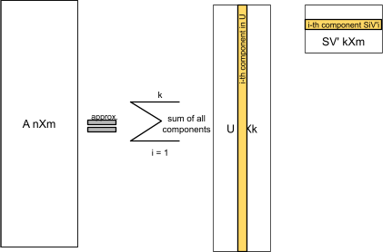
Within this interpretation, we assume that the data generation producing A, is actually the result of the superposition of a number of processes, which only a few are considered of interest. The SVD will discover these underlying processes as independent components, although there may not be necessarily a true correspondence between these components and the exact underlying process. In practice, such correspondence can be found especially for the larger SV’s components.
Constraint / Assumption on data
Under linear algebra theory, SVD imposes to have real Eignevalues and orthogonal Eigenvectors. This is always satisfied for real symetric Matrix, such as these matrices AtA or AAt (ref. spectral decomposition prerequisite for Eigenvalues & vectors).
However, for data analysis purposes, there is additional constraint that each variables should follow approximately a Gaussian distribution. If we have a dataset which presents a set of different clusters or none-normal shape then, from the geometry interpretation, we can see that the new axis will not be so meaningful. The new axis will go along, again, the greatest variance, which in turn may be completely missing the set of clusters present in the dataset.
It is also custom to normalize the data before proceeding with its decomposition. Why? Because the SV magnitude will give an indication as to the importance of each SVs in explaining the variance structure of the dataset. This assumes we choose normalized vectors in V's and U's (vector of unit length), but also that we first normalize the attributes in A .
When attribute within the A dataset are not centered around their mean, the first singular vector v will just point to the longest direction toward the centroid of our data set. This will also affect all remaining singular vector which must be orthogonal to this first one. So to avoid this issue of wrong representation, we normalize all attributes so that their centroid gravitate around the origin.
Also, If we had some attributes with significant difference in range, then during numerical computation these attribute would have greater influence in the factorization process. This normalization can be done in numerous way:
- Taking the z-score of each attribute values (subtracting the mean and dividing by their standard deviation) so that the majority of transformed values will be in the range of -1 to 1. However, this cannot be applied when attribute's distribution are far from Gaussian
- Taking rank where new values take the rank order of their original values.
- other more complex forms.
Note on Categorical attribute:
Similarly we must be careful when converting categorical value to number in order not to convey artificial ordering or spurious correlation when no natural ordering exist for the category. Ways to avoid that:
Similarly we must be careful when converting categorical value to number in order not to convey artificial ordering or spurious correlation when no natural ordering exist for the category. Ways to avoid that:
- Map each category to two variable located in at equal distance along a circle, or yet three variables along a sphere (when number of categories is larger)
- Similar but more complex Mapping into a corner of a generalized tetrahedron (ex. http://arxiv.org/pdf/0711.4452.pdf)
The Application in DM : Data reduction and explanatory
One popular application of SVD in data analysis is to reduce complexity and size of any dataset. The method will allow us to discover a smaller number of factors that can be related to the larger set of original attributes. This is a useful step first toward a better understanding of the inter-correlation structure between the attribute and observations.
Similarly, we can choose voluntarily to ignore some less important components, as these may be considered redundant and offer no important structure in our data analysis. Or yet, we may want to visualize our dataset in a 2 or 3-D view in the best possible way.
Similarly, we can choose voluntarily to ignore some less important components, as these may be considered redundant and offer no important structure in our data analysis. Or yet, we may want to visualize our dataset in a 2 or 3-D view in the best possible way.
A word of caution: in data mining setting involving very large dataset, this method is not so useful as there will be many attributes partially correlated to each others in complex and subtle way. Hence, the discovered factors become hardly interpretable
The Application in DM : Noise reduction
Noise in dataset usually origin and combine from a number of multitude source, which results in adding Gaussian-like variability in our dataset, which has a net effect of increasing the apparent dimensionality of the dataset.
Let’s say we have a few variables which turn out to be highly correlated, adding noise to these observed variables will in fact obscure or the correlation pattern and making the dataset to appear at higher dimensionality than it really is.
The ordering nature of the SV’s value allow us to eliminate the later dimensions offering very little or no structure compared to the prior ones. All SV’s after a certain threshold can then be considered as noise, the challenge is to estimate this threshold (few methods exist, refer to Skillicorn book).
Martin