This post describes Logistic regression (LR) from Machine Learning (ML) point of view. This is self-contained and very little prior knowledge is required.
First, contrary to its name, LR does classification and not a regression. It is used to predict the probability of a 2-class (or binary) outcome variable, based on a number of input features. It can also be extended to cover the more general multi-classes problem.
The problem
In ML, we are interested in estimating (learning) an unknown target function t(x) generating an output y (i.e. y = t(x)), given a number of input variables (or features) represented by vector x of size=d. The premise is that function t is normally quite complex and noisy so that there is no hope in finding its true analytical form. Instead we resort to finding a good function estimate (h(x), as it is often called hypothesis) that should perform well in both in-sample (training) and more importantly out-of-sample (prediction)!
The target t(x) is not a valid function in the mathematical sense: there will likely be different outcome for the same input. Consider any real-life binary outcome that we could be interested in predicting: ’Approve credit’, ‘Team win’, ‘Approve access’, ‘Failure within some period’, etc.. Most outcomes in life are not deterministic and we all accept some level of uncertainty or randomness (stochastic process). This calls for a probabilistic approach giving us the framework for dealing with this.
Our estimate function h should give us some confidence that the outcome will be positive or negative (y ∈{0,1}), given a new input x and parametrized by its parameters (represented by vector θ). This is represented by the probability equations below, obtained from the fact that two outcomes cover all possibilities:
→ p(y = 1 | x; θ) [0,1] = hθ(x)
→ p(y = 0 | x, θ) [0,1] = 1 - hθ(x) (eq. 1)
In ML, we’re aiming to find hθ taken from an Hypothesis set H defining function forms, ex: a set of simple linear, a set of more complex polynomial (2nd, 3rd, 4th degree each being a diferent set), a set complex non-linear form, or even non-tractable form (ex. neural network, support vector machine).
It would be nice if we could use a polynomial form such like hθ(x) = θt x, and leverage derivation done with regression problem. This form implies adding an extra feature xi0 which equals to 1 for all i, so that we can treat the parameter θ0 as the others during optimization.
But there’s no polynomial functions that produce an output y ∈ [0,1] from continuous input variables x, justifying the use of an alternative function representation. This is where a nonlinear function like the Logistic function (sigmoid form) comes to the rescue. whose output y ∈ [0,1] with any input ∈ [-∞,+∞].
Sigmoid function:
If we compose a sigmoid function s(u), such that it takes as input the polynomial u = θt x, and so produces the needed output s(u) = 1 / (1 + e-u), then our hypothesis will output the needed sigmoid values [0,1] :
h(x) = s(θt x) = 11 + exp(-θt x) (eq. 2)
compacting both y classes into a single expression, leads to a convenient way to express the probability function at point (x,y):
p(y | x ; θ) = [11 + exp(-θt x) ] y . [1 - 11 + exp(-θt x)] (1-y) (eq. 3)
This function returns the probability of each class (y=1,0) given the input vector x (new observation) and parametrized by the unknown parameters θ.
|
The interpretation
Using the sigmoid function, it turns out we can interpret its output as genuine probability. The problem is equivalent to “placing” the sigmoid in such a way that it will best separate the input vectors points into two classes. With 3-D geometry, we can imagine a line boundary whose distance with any input points (x1,x2) is calculated by θt x (dot product between point and the line equation) and their estimated probability of being class-1(y=1) is obtained with its vertical distance with the sigmoid (s(θt x)). Such a line boundary is located on the projected line at the center of the sigmoid form (at u=0 and s(u) = ½ ) as illustrated in next figure (ref. http://www.machinelearning.ru/ ):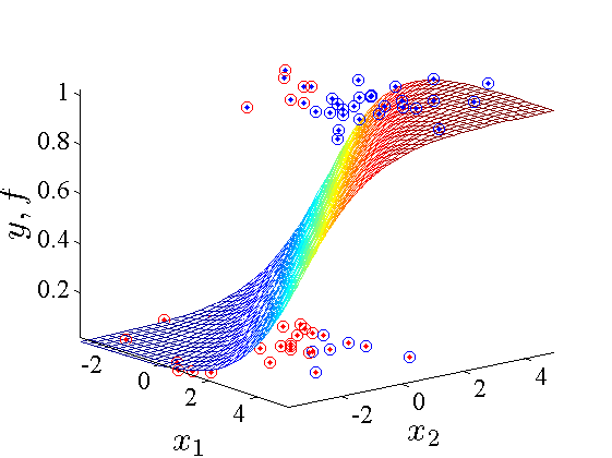
Figure 1. Sigmoid or Logistic function. Boundary line can be imagined by projecting the p=½ probability line (yellow color) into the 2-D plane (x1,x2).
Furthermore, we can easily see how points located far from this boundary will have very large θt x values, resulting in prob ≈ 1 (and conversely: θt x → ∞ ⇒ h ≈ 1, θt x → -∞ ⇒ h ≈ 0), and points near the boundary will have very small distance leading to no clear class (θt x → 0 ⇒ h ≈ ½ ).
The optimal boundary (hyperplane when d>3) will be one where a maximum number of points are correctly classified AND points are on average, located the farthest from it.
But how do we find this location, in other words what are the best estimate for parameters θ? In regression problems, the exact solution is found analytically by minimizing the SSE Error function (sum of squared distance error). A unique solution must exist for θ since a quadratic form is guaranteed to have a unique global minimum (convex form). It turns out the solution found called normal equation also correspond to the most likelihood estimate MLEθ when adopting a probabilistic approach.
However, our issue here is that the sigmoid equation is clearly nonlinear and so will be its associated standard SSE, resulting to potentiel many local minima points typival of non-convex optimization problem. We must abandon the hope to find a closed form solution, and rather use an iterative numerical solution.
But first let’s discover a more suited function to optimize. SSE assumes distance are euclidian-based, but the distance between yi and hi do not makes not much sense with an exponential function like sigmoid, clearly not linear.
To find an alternative optimization function we turn into a probabilistic approach which will give us the best estimate θ or MLE (i.e. Maximum Likelihood estimate). The ML idea poses this question: how likely are we to observe the dataset ⅅ given the function parameters θ, expressed as p(ⅅ | θ) or simply L(θ). This reasoning is a bit counterintuitive, especially considering that our dataset is the only one we have and observable (but this part of a broader debate between frequentist and bayesian and may involve overfitting issues with a limited number of observations).
The ML’s goal is to maximize L(θ) as to find the best suited parameters θ. To calculate L(θ), we assume that each observation point is i.i.d. (independent and identically distributed) random variables x, which is a reasonable condition for most scenario. Note that no restriction is imposed on probability distribution form of our variables x!
Remember the probability of a single observation given in (3), then the Likelihood function of ⅅ is simply the product of probability of all points (each point ), leading to this simplified equation:
L(θ) = i=1,n p(yi | xi ; θ)
Taking log likelihood allows to convert a product over all points to a summation and simplify the rest of the derivation:
l(θ) = log( L(θ) ) = i=1,n log( p(yi | xi ; θ) )
Now expressing with our function we wish to learn hθ(x):
l(θ) = i=1,n yi log(hθ(xi) ) + (1-yi) log(1 - hθ(xi)) (eq. 4)
Maximizing log-likelihood l(θ) or equivalently minimizing its negative form will allow us to find the ML estimate θ (MLE). The negative form divided by number of observations (n) has similar role as SSE for regression, hence interpreted as the Error or Loss function Ɛ of logistic or sometimes called cross-entropy loss:
Ɛ(θ) = -1 n i=1,n yi log(hθ(xi) ) + (1-yi) log(1 - hθ(xi)) (eq. 5)
Let’s continue by minimizing the loss Ɛ(θ) in order to derive the algorithm used by iterative numerical methods like Gradient Descent (or ascent for finding maximum).
Taking partial derivative of (4) leads to,
l(θ)o = l(θ)o 1 ni=1,n -yi log(11 + exp(-θt xi) ) - (1-yi) log(1 - 11 + exp(-θt xi))
l(θ)1 = l(θ)1 1 n i=1,n -yi log(11 + exp(-θt xi) ) - (1-yi) log(1 - 11 + exp(-θt xi))
l(θ)2 = … for and all equivalent partial derivatives for θ2,θ3, .., θd (d+1 equations).
Now to simplify things a bit, we’ll use a single observation (x,y) to ignore the summation because differentiate summation is equivalent to summing a differential. This idea is actually useful when we want to improve Gradient descent performance (ref Stochastic gradient descent below), but for now let’s use this just to simplify the derivation. Re-using the composed function s(u) where u = θt x so to exploit the chained rule in the following way:
l(θ)o= ls{-y log[s(u)]}su{s(u)}uθo(θt x) +ls{-(1-y) log(1-s(u))}su{1- s(u)}uθo(θt x)
…
Recalling the derivative of a sigmoid d(s(u))du= s (1 - s), and obviously uθo(θt x) = x0
l(θ)o = -ys(u)×{s(u)×(1- s(u))} × x0 + (y-1)1 - s(u)×{-s(u)×(1- s(u))} × x0
...
Eliminating some terms, lead simply to,
l(θ)o = {-y × (1- s(u)) + (y-1)× s(u) } × x0
...
Let’s replace s(u) by our hypothesis hθ(x) to have the expression given by x, and put back the summation. After some elimination, we easily show that the partial derivatives with respect to θi turn out to be in very simple:
l(θ)o = i=1,n { hθ(xi) - yi } × xi0
l(θ)1 = i=1,n { hθ(xi) - yi } × xi1 (eqs. 6)
…
where xi0 is the i-th observation of the variable x0 same for xi1 , xi2 , .. xid (feature input space in ℝd).
Setting these equation to 0, and solving for parameters θ would give us the best estimate parameters MLEθ. However as said before there is no closed form for these non-linear form hθ(x).
It is useful to look at equation involving xi0 = 1 for all n points and its solution is trivial. We see that the sum ∑i=1,n hθ(x) is equal to the sum of ∑i=1,n yi all class for which yi=1, in otherword the expected value of our predictor E[hθ(x)] equal to 1/n ∑i=1,n yi. This intuitive result confirms the unbiased likelihood estimate given by the method.
Now let’s define the most simple Gradient Descent (called batch) used to resolve for all d+1 parameters θ, in a simple pseudo-code:
Set default initial parameters θt = {0,0,....}
Iterate
# move each param with its gradient d/d𝜭i descending at a certain learning rate (-𝛂)
θ0(cur) = θ0(prev) - 𝞪 i=1,n {yi - hθ(xi)} × xi0
θ1(cur) = θ1(prev) - 𝞪 i=1,n {yi - hθ(xi)} × xi1
…. for all θi(cur)
|
By starting at an initial params value (any point) and keep iterating toward the direction of largest slope we continue descending by re-assigning θi values to new location.
We refer to it as batch because at each iteration we go over the full summation over all points. It is also advisable to calculate the loss value to appreciate the speed of convergence and adjust the learning rate parameter 𝛂 accordingly. This rate should neither be too small (very low convergence), nor too big (may not decrease on every step or worst may no convergence as it will overshoot). A simple heuristic, is to use small value (eg. 0.001) and increase by a factor of 3 each time (i.e. log-scale as we multiply by 3 from previous values until we converge in an optimal way: 0.01, 0.03, 0.1, 0.3, 1, etc..).
Algorithm optimization
Similar result could be obtained by applying Gradient Descent, on the set of Gradient equations derived from the error function (equation 5) instead of the MLE. It it worthwhile to note that same equations would be found for Gradient of regression problem, only the form or the hypothesis would differ. In fact, this is true for every exponential and is proved by the Generalized Linear Model theory (GLM).
Batch algorithm is the brute force, and there are alternatives:
- Newton-Raphson based on Newton method or its generalized form (d>2)
- Many more exists.
But these are just optimization tricks (part of mathematics called numerical methods) and do not change the nature of the problem.
Martin